Scaling Law

IIya at NeurIPS 2024 gave a talk about his work on SeqtoSeq learning. In this talk, he mentioned about the scaling law of LLM and also pointed out that the pretraing will end soon. Let us dive into the topic of scaling law of LLM. We will first understand what is the scaling law of LLM and then we will see what might be the next.

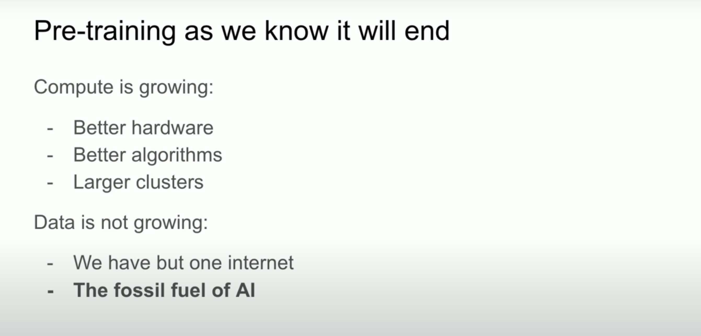
As seen in the above figiure, he noted that the pretraining will eventually reach its limits due to the finite nature of available data, akin to a “fossil fuel” in AI. And also the scaling law is the backbone behind the pre-training. So let us first understand what is the scaling law of LLM.

Scaling Law

As we heard, if we train larger models over more data, we will get better results. Scaling laws help us to quantify the relationship between LLM’s test loss or other performance metrics with some settings of LLM that we are trying to scale including model size, data size and the compute used for training. And in almost all reserach related to scaling laws, the fundamental equation is the power law or more exactly the inverse power law, which can be written as:

\[\text{Performance} = a(\frac{1}{Scale Factor})^{p}\]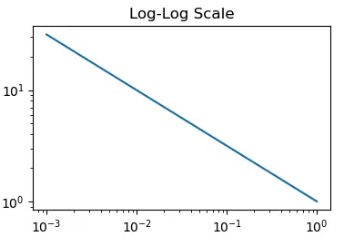

If we plot it via a log scale, we will get a linear line that is visualizing the most LLM scaling laws. And those patterns would be seen in all of studies related to the scaling laws.

The practical usage of scaling laws is to help us make decisions about large-scale model training. Since training massive models requires significant investment (potentially millions of dollars), we need ways to predict performance before committing resources. Scaling laws provide a solution by allowing us to:

1. Train multiple smaller models with different configurations
2. Derive scaling relationships from their performance
3. Extrapolate to predict large model performance

While this approach has limitations since larger models may behave differently than smaller ones, it remains a valuable tool for AI research. The ability to forecast performance gives researchers more confidence in scaling decisions and helps justify continued investment in larger models.

In the following, we will dive into two most well-known studies related to the scaling laws.

Scaling Laws for Neural Language Models

This study is trying to check the relationship between the scale factors and the LLM’s performances ( ). Key findings could be summarized as follows:

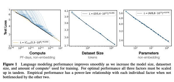
• A power law relationship is observed between those three scale facotrs: model parames, data size and compute used for training and the LLM’s test loss when performance is not bottlenecked by the model shape such as depth and width. It is visualized in the following figure.

• Perf improves most if model size and dataset size are scaled up togehter. Increasing one without the other scaling up leads to diminishing returns. And the size of the dataset does not need to be scaled up as much as the model size. For example, if we scale up the mode size by 8 times, the dataset size only needs to be scaled up by 5 times to prevent overfitting.

• Larger models are more sample efficient than smaller models, take fewer steps / data points to reach same loss. Therefore, pretaining an LLM to convergence is sub-optimal. Instead, we should train a much larger model on less data and stop the training early. However, this suggetion is only optimal in terms of training but it does not capture the inference cost.

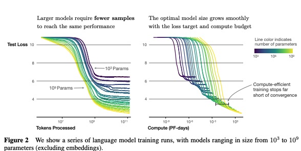
These results show that language modeling performance improves smoothly and predictably as we appropriately scale up model size, data, and compute. We expect that larger language models will perform better and be more sample efficient than current models.

This study is one of the first few studies related to the scaling laws. However, it has the following limitations:

• In the empirical analysis, the learning rate is fixed for all training epochs. While it should be a dynamic which needs to be adjusted based on the number of training steps.
• It suggested scaling model size faster than dataset size, post-GPT-3 studies found that balanced scaling of both parameters and data outperformed models that only increased parameters.

Therefore, we are going to check another study.

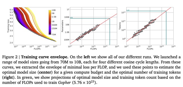
Training Compute-Optimal Large Language Models

In this study, the authors tried to conduct the experiments with much lager models ( Hoffmann 2022). The model size raning from 70M to 17B which are trained over one trillion tokens are checked and compared.

The key findings from this study could be summarized as follows:

• By training LLMs with different model and data size combinations, a power law relationship emerges that predicts test loss. This allows determining optimal training settings for a given compute budget.

• Model and data size should be scaled proportionally for compute-optimal training. This suggests many current LLMs are undertrained - they would benefit from training on much larger datasets. For example, the study predicts Gopher should have used a 20x larger dataset.

• To validate these findings, the authors trained Chinchilla - a 70B parameter model with 1.4T training tokens. Despite being 4x smaller than Gopher, Chinchilla achieved better performance by using more training data with the same evaluation approach.

“The amount of training data that is projected to be needed is far beyond what is currently used to train large models.”

From these two papers, the quick takeaways could be summarized as follow:

• Kaplan’s study suggests that we should scale up the model size faster than the dataset size.
  • With a 100X compute budget, we can scale up the model size by 25X and the dataset size by 4X.
• Hoffmann’s study suggests that we should scale up the model size and dataset size proportionally.
  • With a 100X compute budget, we can scale up the model size by 10X and the dataset size by 10X.

Than, in the recent years, the Hoffmann’s study is more popular and widely used. We can also understand this by the fact that this study is more practical in terms of the inference cost.

The GPT Journey: Proof of Scaling Laws

It is the age of pretraining. In OpenAI and other foundation models, we can see the journey to push the model performances is just train increasingly large models on bigger and higher quality datasets. For example, the creation of OpenAI’s GPT lineage of models is a testament to the scaling laws. This is exactly what happened with GPT-1, GPT-2, GPT-3, and GPT-4.

Since GPT-4 is not open-sourced, we will use the model upto GPT-3 to understand the scaling laws.

Model Version	Architecture	Parameter Count	Training Data
Bert-base	12-level, 12-headed Transformer encoder	0.11 billion	Toronto BookCorpus and English Wikipedia (3,200 million words)
Bert-Large	24-level, 16-headed Transformer encoder	0.34 billion	Toronto BookCorpus and English Wikipedia (3,200 million words)
GPT1	12-level, 12 headed Transformer decoder, followed by linear-softmax	0.12 billion	BookCorpus, 4.5 GB of text
GPT2	GPT-1, but with modified normalization	1.5 billion	WebText: 40 GB of text, 8 million documents
GPT3	GPT-2 but with modification to allow larger scaling	175 billion	570 GB plaintext, 0.4 trillion tokens

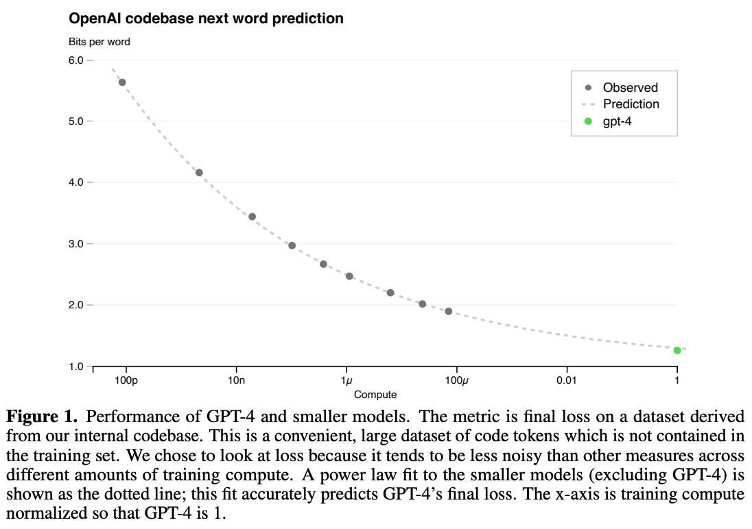
And than, in the GPT-4 technical report, due to the high cost of large-scale pretraining, model-specific tuning is not feasible. Therefore, the authors used scaling laws to predict model performance before training ( Achiam 2023). The key findings could be summarized as follows:

• They trained smaller models using 1,000-10,000x less compute to fit power laws. These power laws were then used to predict the performance of much larger models like GPT-4. The formula is as follows:

\[\text{L(C)} = a(C)^{b} + c\]

where $C$ is the training compute budget, $a$ and $b$ are power law parameters. And c is the irreducible loss term.

• The final loss of properly-trained LLMs follows a power law relationship with compute, with an added irreducible loss term since test loss may never reach zero.

• Using these scaling laws, they were able to predict GPT-4’s final performance with high accuracy. The improvement in loss shows diminishing returns with increased compute.

Therefore, in the GPT journey, we can see the importance of scaling up the pretrainin process. And considering the pretrianing is very expensive, scaling laws make the process more predictable and efficient. You can also think it give us more confidence to invest in the pretraining process.

The End of Scaling Laws/Pretraining?

Let us see what IIlya said in his NIPS talk: pretraining and scaling laws could be hitting the limits. There are some debats over this topic. For example, Sam Altman mentioned that there is no wall.

In a more fair way, we can say even from the scaling laws, we will see it is slowing down. The rate of improvement for users is reducing with the further increase of the scale factors. And in the recent years, we all agree that scaling up LLM pretraining will require that we create larger pretraining datasets. We might run out of data to train LLM models. Right now, companies get most of their training data by copying text from websites. But there’s only one internet. Once we’ve used that data, it will be hard to find new high-quality data to train even larger models. So it is the point that Ilya mentioned in his talk: Compute power is growing rapidly while Data growth is constrained by web scraping limitation. This mismatch means pretraining may hit fundamental limits.

One big challenge with scaling laws is that they assume all training data is equally good. But in reality, there’s only so much high-quality data available. This raises the question of whether synthetic data could help, but current approaches mostly just remix existing information rather than create truly new insights. It’s like we’re hitting a wall - we’ve used up most of the valuable human-created content available for training.

There might be a solution if we use more computing power to generate better synthetic data during testing. While we can’t create more human knowledge out of thin air, we could use GPU processing power to generate higher quality training data. However, this would need much more computing power than originally predicted by scaling laws. The key is finding the right balance between training and testing - they need to work together and also in a smart way. The optimized flow would be: train a model, use scaled-up inference compute to generate rich synthetic data, and then use that data to further improve the model through training. Similar to how humans learn by building on previous knowledge while also creating new insights through real-world experience. Those new insights would be recored in the book to be passed on to the next generation. Maybe this can be the future of LLMs. We will have tons of LLMs or inference processes running every moment and everywhere. Few of smart LLMs will be able to generate high-quality synthetic data to train the next generation of LLMs. Than, it might be the new paradigm of scaling laws.

What is the Future?

If it is not scaling laws, what is the future? The following figure is the answer from IIya at the same talk.

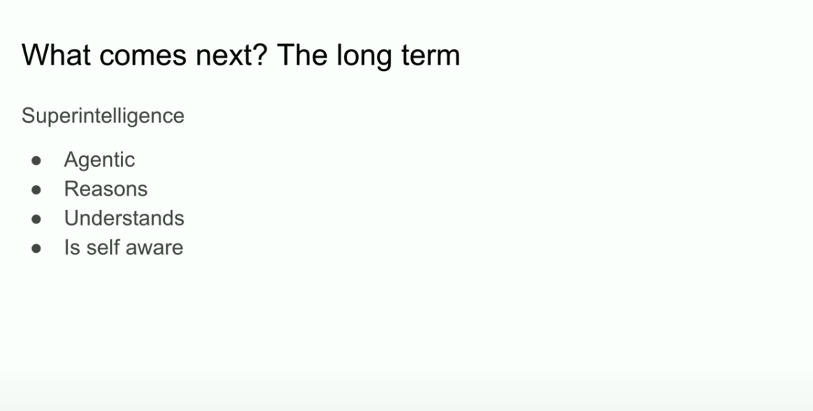
Yes, those are also hot topics now in the LLM community including agents and reasoning models. We will discuss those topics in the coming blogs.

Before the end, we can also quickly disucss one term called FLOPs, which is heavily used in the research of scaling laws.

References

• (). . .
• Hoffmann, Jordan, et al. (2022). Training compute-optimal large language models. arXiv preprint arXiv:2203.15556 . [link]
• Achiam, Josh, et al. (2023). GPT-4 technical report. arXiv preprint arXiv:2303.08774 . [link]

Appendix

What is FLOPs?

It would be better to understand the concept of FLOPs. FLOPs is a measure of the number of floating-point operations required to perform a computation. For example, OpenAI mentioned that it took about 6 FLOP (floating-point operations) per parameter per token to train GPT-4. In terms of LLM’s training, forward and backward passes are all captured by FLOPs. The rule of thumb is that the compute required to train a model is around 6PN FLOPs, where P is the model size and N is the dataset size. And 2PN can capture the forward pass while 4PN can capture the backward pass. The accurate modelling of FLOPs could be found in this blog.

Than, in the scaling law, the compute budget is always defined as values in PetaFLOP-days, or $10^15$ FLOPs/second x 24 hours x 3600 seconds/hour, arriving at $8.64\multiply10^19$ FLOPs.